
.png)
The ATR Channel breakout strategy coded for Trading View
Trend-following can be a very profitable trading method. But this approach is hard to execute: win percentages are typically low and drawdowns excessive. Let’s see and measure how one of those trend-following strategies performs in TradingView.
Trend following with the ATR Channel breakout strategy for TradingView
In Way of the Turtle, Curtis Faith (2007) describes his lessons as one of the original Turtles. In the eighties Turtles were ordinary people trained by Richard Dennis, a very successful trader. He taught them two profitable trend-following strategies and, once they completed their training, gave them an account of up to $2 million to trade. During his Turtle years Faith earned over $30 million for Dennis.
Turtles were trend followers. Trend followers try to profit from large price movements that occur over the span of several months (Faith, 2007). They buy when markets make historical highs and short when prices plummet. For that to work trend followers require price momentum to sustain in the same direction. What makes trend following difficult is that drawdowns can be huge, win percentages low, and missing a couple of big trades can ruin an entire year of trading (Faith, 2007).
One trend-following strategy that Faith (2007) shares in his book is the ATR Channel Breakout strategy. This strategy is a volatility-based system that uses the Average True Range (ATR) as a measure for price fluctuations. For this we plot an upper and lower band based on recent volatility. Those bands make it easier to identify price movements that go beyond the regular trading range and mark the start of a new trend, or so the underlying idea goes.
Let’s see what trading rules that strategy has and how we program it for TradingView.
Trading rules of the ATR Channel breakout strategy
The ATR Channel breakout strategy has the following trading rules (Faith, 2007):
- Enter long rules:
- Open a long position when the close is above the top of the channel, which is computed as follows: 350-day moving average + 7 x the 20-bar Average True Range (ATR).
- Exit long rules:
- Close the long position when prices cross below the 350-day moving average.
- Enter short rules:
- Open a short position when the close is below the bottom of the channel, computed as follows: 350-day moving average - 3 x ATR.
- Exit short rules:
- Cover the short position when prices cross above the 350-day moving average.
- Position sizing:
- For long and short positions, determine the position size by dividing 0.5% of equity by the value of the market’s 20-bar Average True Range (ATR) in terms of dollars.
One thing this strategy lacks is a stop-loss order. However, there is an implicit stop: when prices move against the position, at some point they will cross the 350-day moving average. That will then trigger the strategy’s exit signal. This way losses are limited, but not in the sense that there’s a fixed stop-loss price that we know in advance.
Another thing to note is that Faith (2007) didn’t specify the type of moving average. Based on my interpretation of his book, I assume he uses a Simple Moving Average (SMA).
The profitable backtest that Faith (2007) performed was done on daily data and a wide range of futures markets. The backtested instruments included foreign exchange (Australian dollar, British pound, Euro), commodities (gold, crude oil, copper, natural gas), soft commodities (cotton, coffee, cattle, soybeans), and fixed-income futures (Treasury notes and bonds).
Programming the ATR Channel breakout trading strategy for TradingView
Now that we know the trading rules let’s code the strategy script. A practical way to write strategies is to use a coding template. That breaks up the large task of writing a strategy into smaller, easier-to-manage chunks of work. And it becomes less likely we overlook things. Plus it adds structure to our thinking.
We’ll use the following template to code the ATR Channel Breakout strategy:
//@version=5
// 1. Define strategy settings


// 2. Calculate strategy values


// 3. Output strategy data


// 4. Determine long trading conditions


// 5. Code short trading conditions


// 6. Submit entry orders


// 7. Submit exit orders
If you want to follow along with the article, make a new strategy script in TradingView’s Pine Editor and paste in the above template.
To get an idea of what the code we will write actually does, here’s how the completed strategy looks on the chart:
Now let’s code this strategy for TradingView.

Step 1: Define strategy settings and input options
We first define the strategy’s settings and its input options. For this we use the following code as our first step:
//@version=5
// 1. Define strategy settings
strategy(title="ATR Channel Breakout", overlay=true,
     pyramiding=0, initial_capital=100000,
     commission_type=strategy.commission.cash_per_order,
     commission_value=4, slippage=2)

smaLength = input.int(350, title="SMA Length")
atrLength = input.int(20, title="ATR Length")

ubOffset = input.float(7, title="Upperband Offset", step=0.50)
lbOffset = input.float(3, title="Lowerband Offset", step=0.50)

usePosSize = input.bool(true, title="Use Position Sizing?")
riskPerc   = input.float(0.5, title="Risk %", step=0.25)
We set the script’s settings with the strategy() function. Besides the typical options we use pyramiding to turn off scaling into positions. With initial_capital we set the strategy’s starting funds to 100,000. We set the commission to 4 (commission_value) for each trade (commission_type). With the slippage argument set to 2, stop and market orders are 2 ticks less favourable. (With the commission and slippage pessimistic the strategy really has to prove its worth.)
Next we add the strategy’s input options. The first two input options, ‘SMA Length’ and ‘ATR Length’, are integer inputs made with the input.int() function. We use these for the ATR channel. We give these a default value of 350 and 20.
The next two are floating-point input options that the input.float() function makes. We name these ‘Upperband Offset’ and ‘Lowerband Offset’. They’ll determine how many ATR multiplies the upper and lower band are placed from the average. They get defaults of 7 and 3.
Next is a Boolean true/false input option: ‘Use Position Sizing?’. The input.bool() makes this one. This setting easily toggles the strategy’s position sizing algorithm on or off. We start with using that algorithm (true by default), but if we turn this setting off the strategy will simply trade one contract for each trade.
The ‘Risk %’ is the last input option. This floating-point input (input.float()) defines how much equity the position sizing code uses per trade. It starts with 0.5% risk as the default.
We store the value of each input option in a variable. That way we can reference the input option’s current value later on by simply using the variable.
Step 2: Calculate trading strategy values
For the second step we calculate the strategy’s values:
// 2. Calculate strategy values
smaValue = ta.sma(close, smaLength)
atrValue = ta.atr(atrLength)

upperBand = smaValue + (ubOffset * atrValue)
lowerBand = smaValue - (lbOffset * atrValue)

riskEquity  = (riskPerc / 100) * strategy.equity
atrCurrency = atrValue * syminfo.pointvalue
posSize     = usePosSize ? math.floor(riskEquity / atrCurrency) : 1
First we determine the SMA with TradingView’s ta.sma() function. We have that function run on closing prices (close) for the number of bars set by the smaLength input variable. Then we calculate the ATR with the ta.atr() function and the atrLength input variable. We store these two computed values in the smaValue and atrValue variables.
Next we calculate the ATR channel’s upper and lower band. For the upper band we increase the SMA with the ATR value multiplied by ubOffset, the input variable we gave a default of 7. To arrive at the lower band’s value we decrease the SMA with lbOffset times the ATR. We store these band values in the upperBand and lowerBand variables.
Then we calculate the position size. The algorithm that Faith (2007) uses has two components: a percentage of equity and the ATR in currency value. The first part has us divide riskPerc with 100. That translates the percentage-based input option into a decimal value (so 0.5% becomes 0.005). Then we multiply with strategy.equity, a variable that returns the strategy’s current equity (that is, initial capital + accumulated net profit + open position profit) (TradingView, n.d.).
To determine the currency value of the ATR we multiply atrValue with syminfo.pointvalue. That TradingView variable returns the point value for the current instrument (TradingView, n.d.). For instance, for the E-mini S&P this variable returns 50 since one point of price movement in ES is worth $50. For crude oil futures, which have an underlying of 1,000 barrels, syminfo.pointvalue returns 1,000.
The posSize variable we make next holds the strategy’s position size. Here we have the conditional operator (?:) check if the usePosSize input variable is true. When it is, we divide the risk equity with the ATR currency value. Then we use the math.floor() function to round the position size down to the nearest full integer. Should that input variable be false, however, we simply set posSize to 1. That has us always trade one contract when the position sizing input is turned off.
Step 3: Output the strategy’s data and visualise signals
To make it easier to validate the strategy, we plot its data on the chart next:
// 3. Output strategy data
plot(smaValue, title="SMA", color=color.orange)
plot(upperBand, title="UB", color=color.green, linewidth=2)
plot(lowerBand, title="LB", color=color.red, linewidth=2)
We show the strategy’s values on the chart with TradingView’s plot() function. The first plot() statement shows the 350-day moving average (smaValue). We name that plot ‘SMA’ and colour it color.orange.
The next two plot() function calls show the ATR channel’s upper and lower band on the chart. We show upperBand values in the color.green colour and have lowerBand values show with the color.red colour value. With the linewidth argument set to 2 these line plots are a bit thicker than normal.
Step 4: Code the long trading rules
Next up are the conditions that determine when we open and exit long positions. From the trading rules above we know that the strategy goes long when the close breaks above the channel’s upper band. And long positions are closed when prices go below the simple moving average.
Here’s how we translate that into code:
// 4. Determine long trading conditions
enterLong = ta.crossover(close, upperBand)
exitLong  = ta.crossunder(close, smaValue)
The first Boolean variable we make here, enterLong, gets its true/false value from ta.crossover(). That built-in function returns true when the value of its first argument crossed above that of the second argument (TradingView, n.d.). Here we have the function check if the instrument’s closing prices (close) cross above the ATR channel’s upper band (upperBand). This makes enterLong true when prices break above the channel and false when they don’t.
The exitLong Boolean variable gets its value with the ta.crossunder() function. That function returns true when the value of its first argument dropped below that of the second argument (TradingView, n.d.). We run that function on closing prices and the 350-bar SMA (smaValue). This way exitLong is true when prices break above the moving average. When that situation doesn’t happen on the current bar, exitLong is false.
Step 5: Program the short trading conditions
Then we calculate the short conditions. As the trading rules mentioned, we go short when prices close below the lower ATR channel band. And we exit shorts when prices move above the SMA.
In code those conditions look like:
// 5. Code short trading conditions
enterShort = ta.crossunder(close, lowerBand)
exitShort  = ta.crossover(close, smaValue)
We set the enterShort Boolean variable with ta.crossunder(). Here we have the function check if closing prices (close) dropped below the ATR channel (lowerBand). When they did, the variable is true. Otherwise, false is the variable’s value.
We code the exitShort variable so that it monitors whether the closing prices get above the SMA (smaValue). This we measure with the ta.crossover() function. When they do, the variable is true and else its value is false.
Step 6: Open a trading position with entry orders
Next we use the true/false variables from the previous steps to open long and short positions:
// 6. Submit entry orders
if enterLong
    strategy.entry("EL", strategy.long, qty=posSize)

if enterShort
    strategy.entry("ES", strategy.short, qty=posSize)
The first if statement checks whether enterLong is true. When it is, the strategy.entry() function opens a long position (strategy.long). We give that order the ‘EL’ identifier. And use the posSize variable to define the order’s quantity. Given how we coded that variable earlier, it either holds an ATR-based risk of 0.5% equity or a default position size of 1 contract.
The other if statement evaluates enterShort. When that variable is true during the current script calculation, strategy.entry() submits an enter short order (strategy.short). We name that order ‘ES’ and submit it for posSize contracts.
Step 7: Close market positions with exit orders
Then we need to specify when the strategy should exit positions. We use this code for that:
// 7. Submit exit orders
if exitLong
    strategy.close("EL")

if exitShort
    strategy.close("ES")
The first if statement test whether the exitLong variable is true. This happens when the close drops below the moving average. In that situation, we call the strategy.close() function to close the "EL" entry order.
The second if statement evaluates whether the exitShort variable is true. That happens when prices cross above the SMA. In that scenario, strategy.close() closes the "ES" entry order.
By the way, the strategy.close() function only comes into effect when there is an open order with the specified ID (TradingView, n.d.). Say we’re short and for whatever reason exitLong becomes true. In that case strategy.close() will not close our short position; it only exits based on exitLong when there’s an open long order, not open short position.
Now that we coded all the strategy’s parts, let’s take a quick view at the strategy’s performance.
Performance of the ATR Channel Breakout strategy for TradingView
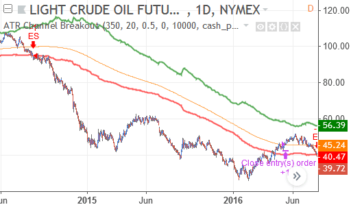
Let’s start with the positive: the ATR Channel Breakout strategy performs very well during long-term trends. Here, for instance, the strategy traded a multi-year downtrend in crude oil futures when prices more than halved:
The strategy also has its weak points. When prices move sideways, the ATR Channel Breakout strategy gets caught up in the chop and incurs losing trade after losing trade. This is, however, a feature that many trend-following strategies share.
In this sideways market the strategy didn’t have a winning trade for several years:
The table below shows the strategy’s backtest performance on two instruments. These results are with position sizing disabled. When the strategy did size positions based on Faith’s (2007) algorithm, trading would on some instruments stop before the end of the backtest (because of insufficient capital). But the more trades there are in a backtest, the better we can draw conclusions of the strategy’s performance. And so I performed the tests with position sizing off.
| Performance metric | Crude oil (CL) | Soybean (ZS) |
|---|---|---|
| First trade | 1984-08-30 | 1971-08-11 |
| Last trade | 2017-06-07 | 2018-01-22 |
| Time frame | 1 day | 1 day |
| Net profit | -$8,278 | -$62,731 |
| Gross profit | $119,264 | $91,564 |
| Gross loss | -$127,542 | -$154,295 |
| Max drawdown | $64,000 | $72,269 |
| Profit factor | 0.935 | 0.593 |
| Total trades | 41 | 68 |
| Winning trades | 12 | 17 |
| Win percentage | 29% | 25% |
| Avg trade | -$201 | -$922 |
| Avg win trade | $9,938 | $5,386 |
| Avg losing trade | -$4,398 | -$3,025 |
| Win/loss ratio | 2.26 | 1.78 |
| Commission paid | $332 | $548 |
| Slippage per order | 2 ticks | 2 ticks |
Ideas to improve the ATR Channel Breakout strategy
As the results above show, the performance of the ATR Channel Breakout strategy can definitely use some improvement. Here are some ideas you might find valuable to experiment with:
- The strategy experienced wild swings in equity, partly because of the long-term moving average of 350 bars on a daily chart. Perhaps the strategy can respond quicker to (failed) trends on a lower time frame and/or with a moving average that doesn’t use that many bars.
- Faith (2007) didn’t discuss why he choose the parameter settings that he did. It also isn’t clear why the upper band is based on 7 times the ATR while the lower band uses 3 times the ATR. The strategy might perform better with other parameters, especially when they suit the instrument and chart’s time frame.
- A trend filter would definitely improve the strategy. That helps to not open positions when the market moves sideways, which in turn prevents a lot losing trades.
- The strategy didn’t use stop-loss orders, but only an implicit stop: positions were closed when prices crossed the 350-bar moving average. But the strategy probably doesn’t have to wait until prices cross that moving average before it knows the position isn’t going anywhere. Furthermore, the strategy might bring more peace of mind when we know there’s an actual stop order in the market. So an experiment with stop-loss orders seems appropriate.
- Perhaps the strategy also becomes better with risk management. We can, for example, limit the strategy’s drawdown. Or place a cap on the position size. See the risk management category for other ideas.
Complete code of the ATR Channel breakout strategy for TradingView
The full code of the ATR Channel Breakout strategy is below. Refer to the discussion above for details about specific parts.
//@version=5
// 1. Define strategy settings
strategy(title="ATR Channel Breakout", overlay=true,
     pyramiding=0, initial_capital=100000,
     commission_type=strategy.commission.cash_per_order,
     commission_value=4, slippage=2)

smaLength = input.int(350, title="SMA Length")
atrLength = input.int(20, title="ATR Length")

ubOffset = input.float(7, title="Upperband Offset", step=0.50)
lbOffset = input.float(3, title="Lowerband Offset", step=0.50)

usePosSize = input.bool(true, title="Use Position Sizing?")
riskPerc   = input.float(0.5, title="Risk %", step=0.25)

// 2. Calculate strategy values
smaValue = ta.sma(close, smaLength)
atrValue = ta.atr(atrLength)

upperBand = smaValue + (ubOffset * atrValue)
lowerBand = smaValue - (lbOffset * atrValue)

riskEquity  = (riskPerc / 100) * strategy.equity
atrCurrency = atrValue * syminfo.pointvalue
posSize     = usePosSize ? math.floor(riskEquity / atrCurrency) : 1

// 3. Output strategy data
plot(smaValue, title="SMA", color=color.orange)
plot(upperBand, title="UB", color=color.green, linewidth=2)
plot(lowerBand, title="LB", color=color.red, linewidth=2)

// 4. Determine long trading conditions
enterLong = ta.crossover(close, upperBand)
exitLong  = ta.crossunder(close, smaValue)

// 5. Code short trading conditions
enterShort = ta.crossunder(close, lowerBand)
exitShort  = ta.crossover(close, smaValue)

// 6. Submit entry orders
if enterLong
    strategy.entry("EL", strategy.long, qty=posSize)

if enterShort
    strategy.entry("ES", strategy.short, qty=posSize)

// 7. Submit exit orders
if exitLong
    strategy.close("EL")

if exitShort